Computation of azimuthal Doppler centroid
Lets call \(rg\) and \(az\) as respectively the range and azimuth spatial vectors associated with the selected image. \(rg = \text{sample}\times d_{rg}\) and \(az = \text{line}\times d_{az}\) where \(d_{rg}\) and \(d_{az}\) are respectively the sample and line spacing in meters. The azimuthal Doppler spectrum writes:
The azimuthal Doppler centroid is the mean azimuth frequency of the azimuthal Doppler spectrum. In order to get a good estimation of the Doppler centroid, the average of the Doppler spectrum is computed on the range direction:
(5)\[\textbf{Azimuthal Doppler spectrum}\]
|
|---|
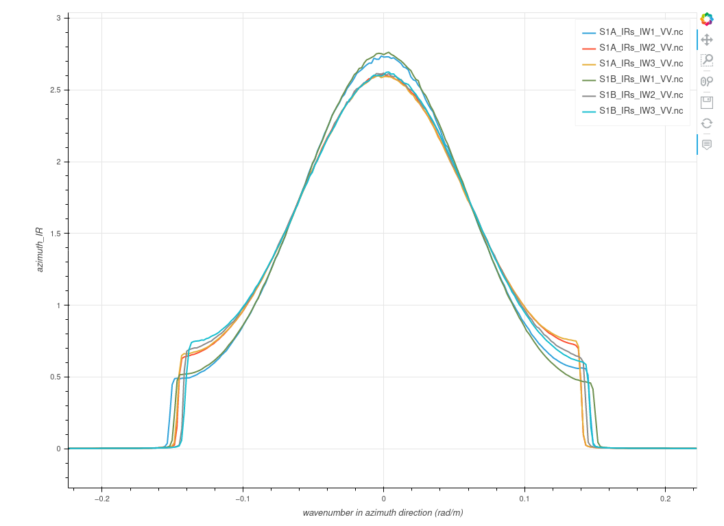
figure (5):Example of Doppler spectrum. |
The azimuthal Doppler centroid is, by definition, the mean (first order moment) of the Doppler spectrum, namely:
However, since the azimuthal Doppler spectrum is not symmetric due to windowing processing applied during the generation of the L1 SLC the estimation of the DC using equation (6) is biased. In practise, the DC is computed by fitting a Gaussian curve on the Doppler spectrum to find the position of the maximum.
Note
This should be updated in the future.
Computation of centered and normalized Doppler spectrum
The that the Doppler spectrum is not centered around zero nor symmetric relatively to its maximum. Several explanations can be given to explain this two characteristics. The not centered value of the azimuthal centroid can be due, among others, to some geophysical aspects such as the observed scene mean motion but also on some instrument uncorrected geometry and uncompensated antenna properties.
The disymmetric shape can also be due to some uncompensated instrument effect but also on applied signal processing such as windowing or interpolation.
In order to correctly further process the Doppler spectrum, it is mandatory to compensate as much as possible these effects with a two step processing:
centering the Doppler spectrum
Normalize the Doppler spectrum by the Impulse Response of the instrument
Centering the Doppler spectrum
Centering the Doppler spectrum and computing the 2D Fourier Transform of the complex modulation signal writes:
Normalization of the Doppler spectrum by the Impulse Response of the instrument
These Impulse Responses have been computed over homogeneous and motion-less surfaces, averaged and stored.
The dataset used to compute theses response is available here and the numerical code to produce them refers to xsarslc.processing.impulseResponse.compute_IR .
The normalization of the doppler spectrum is performed by xsarslc.processing.intraburst.compute_looks method.
(8)\[\textbf{Range Doppler spectrum IW VV}\]
|
|---|

figure (8) :Example of Doppler spectrum along range. |
(9)\[\textbf{Azimuth Doppler spectrum WV VV}\]
|
|---|
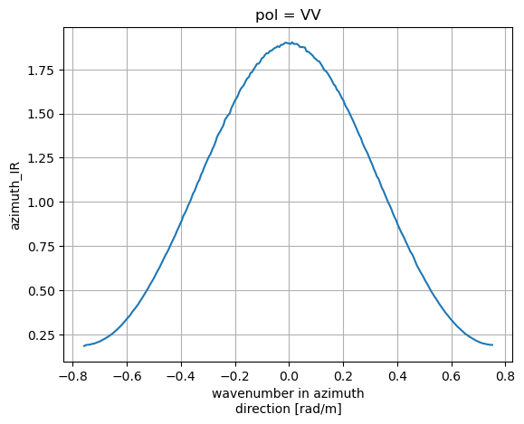
figure (9) :Example of Doppler spectrum along azimuth. |
(10)\[\textbf{Range Doppler spectrum WV VV}\]
|
|---|
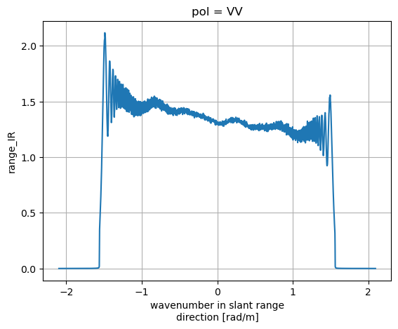
figure (10) :Example of Doppler spectrum along range. |
The normalization with the instrument Impulse Response is realized in the Fourier domain and writes:
with \(IR_{rg}\) and \(IR_{az}\) being the Impulse Response in range and azimuth direction for the considered acquisition mode.
Note
in xsarslc library the methods to estimate the Impulse Response are xsarslc.processing.impulseResponse.compute_IWS_subswath_Impulse_Response() and xsarslc.processing.impulseResponse.compute_WV_Impulse_Response()