Download this notebook from github.
A notebook to illustrate how to compute and correct Impulse Response in WV SLC product
[1]:
"""
This is an example to show how to compute sensor Impulse Response (RI) on WV SLC data
and then correct it.
"""
[1]:
'\nThis is an example to show how to compute sensor Impulse Response (RI) on WV SLC data\nand then correct it.\n'
read a WV SLC over homogeneous region in the rain forest
[2]:
import warnings
warnings.filterwarnings("ignore")
from xsarslc.processing.impulseResponse import generate_WV_AUX_file_ImpulseReponse
# SENTINEL1_DS:/home/datawork-cersat-public/cache/project/mpc-sentinel1/data/esa/sentinel-1a/L1/WV/S1A\_WV\_SLC\_\_1S/2018/050/S1A\_WV\_SLC\_\_1SSV\_20180219T221522\_20180219T222851\_020681\_0236CE\_8F55.SAFE:WV_051
subswathes = {'/home/datawork-cersat-public/cache/project/mpc-sentinel1/data/esa/sentinel-1a/L1/WV/S1A_WV_SLC__1S/2018/050/S1A_WV_SLC__1SSV_20180219T221522_20180219T222851_020681_0236CE_8F55.SAFE':['051'],
             '/home/datawork-cersat-public/cache/project/mpc-sentinel1/data/esa/sentinel-1a/L1/WV/S1A_WV_SLC__1S/2018/062/S1A_WV_SLC__1SSV_20180303T221522_20180303T222851_020856_023C59_7FBF.SAFE':['051']}

IRs = generate_WV_AUX_file_ImpulseReponse(subswathes)
IRs
[2]:
<xarray.Dataset>
Dimensions:         (k_srg: 2048, k_az: 256)
Coordinates:
    pol             <U2 'VV'
  * k_srg           (k_srg) float64 -2.098 -2.096 -2.094 ... 2.092 2.094 2.096
  * k_az            (k_az) float64 -0.7575 -0.7516 -0.7457 ... 0.7457 0.7516
Data variables:
    range_IR        (k_srg) float64 0.0004371 0.0004377 ... 0.0004373 0.0004375
    mean_incidence  float64 23.96
    azimuth_IR      (k_az) float64 0.1835 0.1885 0.1899 ... 0.191 0.1896 0.1897
Attributes:
    long_name:              Impulse response in range direction
    product:                SLC
    swath:                  WV
    multidataset:           False
    ipf:                    2.84
    platform:               SENTINEL-1A
    pols:                   VV
    coverage:               20km * 20km (line * sample )
    orbit_pass:             Ascending
    radar_frequency:        5405000704.0
azimuth_time_interval: 0.0006059988896297211[3]:
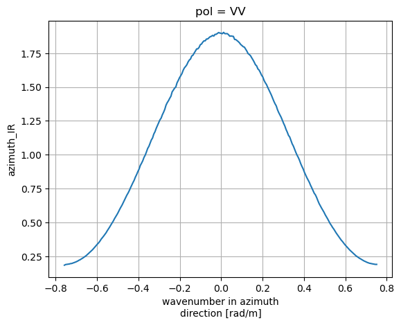
from matplotlib import pyplot as plt
IRs['azimuth_IR'].plot()
plt.grid(True)
[4]:
IRs['range_IR'].plot()
plt.grid(True)

write a netCDF AUX IR file
[5]:
out_file = "/tmp/S1_IR_WV_AUX_FILE.nc"
if 'footprint' in IRs.attrs:
    IRs.attrs.update({'footprint': str(IRs.footprint)})
if 'multidataset' in IRs.attrs:
    IRs.attrs.update({'multidataset': str(IRs.multidataset)})
IRs.to_netcdf(out_file)
print(out_file)
IRs.to_netcdf(out_file)
print(out_file)
/tmp/S1_IR_WV_AUX_FILE.nc
/tmp/S1_IR_WV_AUX_FILE.nc
apply IR correction when computing cross spectra on a WV image
[6]:
out_file = "/tmp/S1_IR_WV_AUX_FILE.nc"
import os
import xsar
import warnings
warnings.filterwarnings("ignore")
#a_wv_safe = '/home/datawork-cersat-public/cache/project/mpc-sentinel1/data/esa/sentinel-1a/L1/WV/S1A_WV_SLC__1S/2023/030/S1A_WV_SLC__1SSV_20230130T095609_20230130T100149_047011_05A391_E93C.SAFE'
a_wv_tiff = '/home/datawork-cersat-public/cache/project/mpc-sentinel1/data/esa/sentinel-1a/L1/WV/S1A_WV_SLC__1S/2023/030/S1A_WV_SLC__1SSV_20230130T095609_20230130T100149_047011_05A391_E93C.SAFE/measurement/s1a-wv1-slc-vv-20230130t100004-20230130t100007-047011-05a391-017.tiff'
fullpathsafeSLC = os.path.dirname(os.path.dirname(a_wv_tiff))
print(fullpathsafeSLC,os.path.exists(fullpathsafeSLC))

imagette_number = os.path.basename(a_wv_tiff).split('-')[-1].replace('.tiff','')
str_gdal = 'SENTINEL1_DS:%s:WV_%s'%(fullpathsafeSLC,imagette_number)
print('str_gdal',str_gdal)
s1ds = xsar.Sentinel1Dataset(str_gdal)
s1ds
/home/datawork-cersat-public/cache/project/mpc-sentinel1/data/esa/sentinel-1a/L1/WV/S1A_WV_SLC__1S/2023/030/S1A_WV_SLC__1SSV_20230130T095609_20230130T100149_047011_05A391_E93C.SAFE True
str_gdal SENTINEL1_DS:/home/datawork-cersat-public/cache/project/mpc-sentinel1/data/esa/sentinel-1a/L1/WV/S1A_WV_SLC__1S/2023/030/S1A_WV_SLC__1SSV_20230130T095609_20230130T100149_047011_05A391_E93C.SAFE:WV_017
[6]:
<Sentinel1Dataset full coverage object>
[7]:
slc = s1ds.datatree['measurement'].to_dataset()['digital_number']
slc
[7]:
<xarray.DataArray 'digital_number' (pol: 1, line: 4907, sample: 5571)>
dask.array<open_rasterio-034951840d7c4223938c19b8c7bd4376<this-array>, shape=(1, 4907, 5571), dtype=complex64, chunksize=(1, 4907, 5000), chunktype=numpy.ndarray>
Coordinates:
  * line     (line) int64 0 1 2 3 4 5 6 7 ... 4900 4901 4902 4903 4904 4905 4906
  * sample   (sample) int64 0 1 2 3 4 5 6 ... 5564 5565 5566 5567 5568 5569 5570
  * pol      (pol) object 'VV'
Attributes:
    comment:  denoised digital number, read at full resolution
history: digital_number: measurement/s1a-wv1-slc-vv-20230130t100004-2023...[8]:
s1ds.dataset
[8]:
<xarray.Dataset>
Dimensions:         (line: 4907, sample: 5571, pol: 1)
Coordinates:
  * line            (line) int64 0 1 2 3 4 5 6 ... 4901 4902 4903 4904 4905 4906
  * sample          (sample) int64 0 1 2 3 4 5 ... 5565 5566 5567 5568 5569 5570
  * pol             (pol) object 'VV'
Data variables:
    digital_number  (pol, line, sample) complex64 dask.array<chunksize=(1, 4907, 5000), meta=np.ndarray>
    time            (line) datetime64[ns] 2023-01-30T10:00:04.057309952 ... 2...
    sampleSpacing   float64 1.498
    lineSpacing     float64 4.144
Attributes: (12/15)
    name:              SENTINEL1_DS:/home/datawork-cersat-public/cache/projec...
    short_name:        SENTINEL1_DS:S1A_WV_SLC__1SSV_20230130T095609_20230130...
    product:           SLC
    safe:              S1A_WV_SLC__1SSV_20230130T095609_20230130T100149_04701...
    swath:             WV
    multidataset:      False
    ...                ...
    start_date:        2023-01-30 10:00:04.057288
    stop_date:         2023-01-30 10:00:07.030318
    footprint:         POLYGON ((130.822283515509 -41.56791070616844, 131.065...
    coverage:          20km * 21km (line * sample )
    orbit_pass:        Ascending
platform_heading: -13.8309692949357[9]:
# from xsarslc.processing.xspectra.compute_subswath_intraburst_xspectra import compute_intraburst_xspectrum
# compute_intraburst_xspectrum(slc, mean_incidence, slant_spacing, azimuth_spacing, synthetic_duration,
#                                  azimuth_dim='line', nperseg={'sample': 512, 'line': 512},
#                                  noverlap={'sample': 256, 'line': 256}, IR_path=out_file)
compute xspec without IR correction
[10]:
from xsarslc.processing.xspectra import compute_WV_intraburst_xspectra
import time
t0 = time.time()
xs0 = compute_WV_intraburst_xspectra(dt=s1ds.datatree,
                                          polarization='VV',periodo_width={"line":3000,"sample":3000},
                                          periodo_overlap={"line":-3000,"sample":-3000})
print('time to compute x-spectra on WV :%1.1f sec'%(time.time()-t0))
xs0
time to compute x-spectra on WV :157.2 sec
[10]:
<xarray.Dataset>
Dimensions:                   (bt_thresh: 5, 0tau: 3, freq_line: 145,
                               freq_sample: 397, 1tau: 2, 2tau: 1, c_sample: 2,
                               c_line: 2, k_gp: 4, phi_hf: 5,
                               lambda_range_max_macs: 10)
Coordinates:
    pol                       <U2 'VV'
  * bt_thresh                 (bt_thresh) int64 5 50 100 150 200
    k_rg                      (freq_sample) float64 0.0 0.002094 ... 0.829
    k_az                      (freq_line) float64 -0.1506 -0.1485 ... 0.1506
    line                      int64 2453
    sample                    int64 2785
    longitude                 float64 130.9
    latitude                  float64 -41.45
  * k_gp                      (k_gp) int64 1 2 3 4
  * phi_hf                    (phi_hf) int64 1 2 3 4 5
  * lambda_range_max_macs     (lambda_range_max_macs) float64 50.0 ... 275.0
Dimensions without coordinates: 0tau, freq_line, freq_sample, 1tau, 2tau,
                                c_sample, c_line
Data variables: (12/26)
    incidence                 float64 23.31
    ground_heading            float64 -15.36
    sensing_time              datetime64[ns] 2023-01-30T10:00:05.543825664
    sigma0                    float64 0.368
    nesz                      float64 0.001408
    bright_targets_histogram  (bt_thresh) int64 539 0 0 0 0
    ...                        ...
    corner_line               (c_line) int64 25 4881
    corner_sample             (c_sample) int64 25 5545
    burst_corner_longitude    (c_sample, c_line) float64 130.8 130.8 131.1 131.0
    burst_corner_latitude     (c_sample, c_line) float64 -41.57 ... -41.34
    cwave_params              (k_gp, phi_hf, 2tau) float64 7.757 ... -0.1919
    macs                      (lambda_range_max_macs, 2tau) complex128 (0.329...
Attributes: (12/21)
    name:                   SENTINEL1_DS:/home/datawork-cersat-public/cache/p...
    short_name:             SENTINEL1_DS:S1A_WV_SLC__1SSV_20230130T095609_202...
    product:                SLC
    safe:                   S1A_WV_SLC__1SSV_20230130T095609_20230130T100149_...
    swath:                  WV
    multidataset:           False
    ...                     ...
    radar_frequency:        5405000704.0
    azimuth_time_interval:  0.0006059988896297211
    tile_width_line:        20125.523484
    tile_width_sample:      <xarray.DataArray 'cumulative ground length' ()>\...
    tile_overlap_sample:    0.0
tile_overlap_line: 0.0compute xspec with IR corretion
[11]:
import time
import xsarslc.processing.xspectra
from importlib import reload
reload(xsarslc.processing.xspectra)
t0 = time.time()
xs1 = xsarslc.processing.xspectra.compute_WV_intraburst_xspectra(dt=s1ds.datatree,
                                          polarization='VV',periodo_width={"line":3000,"sample":3000},
                                          periodo_overlap={"line":-3000,"sample":-3000},IR_path=out_file)
print('time to compute x-spectra on WV :%1.1f sec'%(time.time()-t0))
xs1
time to compute x-spectra on WV :186.6 sec
[11]:
<xarray.Dataset>
Dimensions:                   (bt_thresh: 5, 0tau: 3, freq_line: 145,
                               freq_sample: 397, 1tau: 2, 2tau: 1, c_sample: 2,
                               c_line: 2, k_gp: 4, phi_hf: 5,
                               lambda_range_max_macs: 10)
Coordinates:
    pol                       <U2 'VV'
  * bt_thresh                 (bt_thresh) int64 5 50 100 150 200
    k_rg                      (freq_sample) float64 0.0 0.002094 ... 0.829
    k_az                      (freq_line) float64 -0.1506 -0.1485 ... 0.1506
    line                      int64 2453
    sample                    int64 2785
    longitude                 float64 130.9
    latitude                  float64 -41.45
  * k_gp                      (k_gp) int64 1 2 3 4
  * phi_hf                    (phi_hf) int64 1 2 3 4 5
  * lambda_range_max_macs     (lambda_range_max_macs) float64 50.0 ... 275.0
Dimensions without coordinates: 0tau, freq_line, freq_sample, 1tau, 2tau,
                                c_sample, c_line
Data variables: (12/26)
    incidence                 float64 23.31
    ground_heading            float64 -15.36
    sensing_time              datetime64[ns] 2023-01-30T10:00:05.543825664
    sigma0                    float64 0.368
    nesz                      float64 0.001408
    bright_targets_histogram  (bt_thresh) int64 539 0 0 0 0
    ...                        ...
    corner_line               (c_line) int64 25 4881
    corner_sample             (c_sample) int64 25 5545
    burst_corner_longitude    (c_sample, c_line) float64 130.8 130.8 131.1 131.0
    burst_corner_latitude     (c_sample, c_line) float64 -41.57 ... -41.34
    cwave_params              (k_gp, phi_hf, 2tau) float64 7.733 ... -0.1993
    macs                      (lambda_range_max_macs, 2tau) complex128 (0.327...
Attributes: (12/21)
    name:                   SENTINEL1_DS:/home/datawork-cersat-public/cache/p...
    short_name:             SENTINEL1_DS:S1A_WV_SLC__1SSV_20230130T095609_202...
    product:                SLC
    safe:                   S1A_WV_SLC__1SSV_20230130T095609_20230130T100149_...
    swath:                  WV
    multidataset:           False
    ...                     ...
    radar_frequency:        5405000704.0
    azimuth_time_interval:  0.0006059988896297211
    tile_width_line:        20125.523484
    tile_width_sample:      <xarray.DataArray 'cumulative ground length' ()>\...
    tile_overlap_sample:    0.0
tile_overlap_line: 0.0compare with/without
[12]:
import numpy as np
from xsarslc.processing import xspectra
xs = xs0.swap_dims({'freq_line': 'k_az', 'freq_sample': 'k_rg'})
xs = xspectra.symmetrize_xspectrum(xs['xspectra_2tau'], dim_range='k_rg', dim_azimuth='k_az')
xs_ir = xs1.swap_dims({'freq_line': 'k_az', 'freq_sample': 'k_rg'})
xs_ir = xspectra.symmetrize_xspectrum(xs_ir['xspectra_2tau'], dim_range='k_rg', dim_azimuth='k_az')
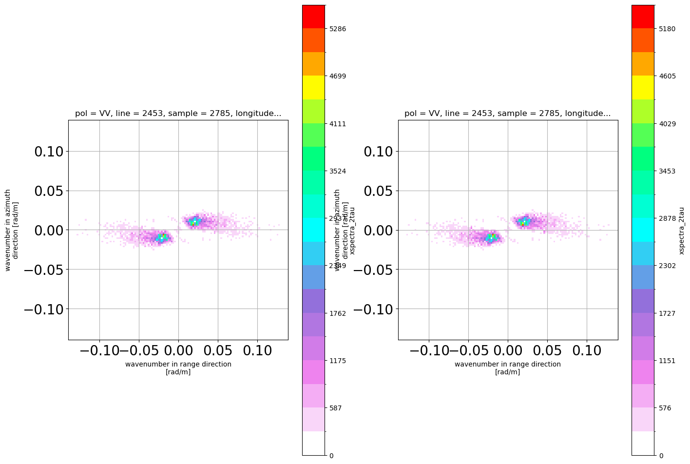
############################################ real part ############################
coS=np.abs(xs.mean(dim='2tau').real) # co spectrum = real part of cross-spectrum
coS_reduced = coS.where(np.logical_and(np.abs(coS.k_rg)<=0.14, np.abs(coS.k_az)<=0.14), drop=True)
coS_IRcor=np.abs(xs_ir.mean(dim='2tau').real) # co spectrum = real part of cross-spectrum
coS_reduced_IRcor = coS_IRcor.where(np.logical_and(np.abs(coS_IRcor.k_rg)<=0.14, np.abs(coS_IRcor.k_az)<=0.14), drop=True)
from matplotlib import pyplot as plt
%matplotlib inline
from matplotlib import colors as mcolors
cmap = mcolors.LinearSegmentedColormap.from_list("", ["white","violet","mediumpurple","cyan","springgreen","yellow","red"])
PuOr = plt.get_cmap('PuOr')
plt.figure(figsize=(16,12))
plt.subplot(1,2,1)
#coS_reduced_av=coS_reduced.rolling(k_rg=3, center=True).mean().rolling(k_az=3, center=True).mean()
coS_reduced.plot(cmap=cmap, levels=20, vmin=0)
plt.grid()
plt.xticks(fontsize=20)
plt.yticks(fontsize=20)
plt.axis('scaled')
plt.subplot(1,2,2)
#coS_reduced_av=coS_reduced.rolling(k_rg=3, center=True).mean().rolling(k_az=3, center=True).mean()
plt.title('with IR correction')
coS_reduced_IRcor.plot(cmap=cmap, levels=20, vmin=0)
plt.grid()
plt.xticks(fontsize=20)
plt.yticks(fontsize=20)
plt.axis('scaled')
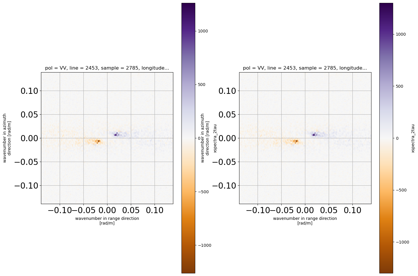
############################################ imag.part ############################
ims = xs.mean(dim='2tau').imag.squeeze()
xS_red = ims.where(np.logical_and(np.abs(ims.k_rg)<=0.14, np.abs(ims.k_az)<=0.14), drop=True)
ims_irCor = xs_ir.mean(dim='2tau').imag.squeeze()
xS_red_IRCor = ims_irCor.where(np.logical_and(np.abs(ims_irCor.k_rg)<=0.14, np.abs(ims_irCor.k_az)<=0.14), drop=True)
#xS_av=xS_red.rolling(k_rg=3, center=True).mean().rolling(k_az=3, center=True).mean()
plt.figure(figsize=(16,12))
plt.subplot(1,2,1)
xS_red.plot(x='k_rg',cmap=PuOr)
plt.grid()
plt.xticks(fontsize=20)
plt.yticks(fontsize=20)
plt.axis('scaled')
plt.subplot(1,2,2)
xS_red_IRCor.plot(x='k_rg',cmap=PuOr)
plt.grid()
plt.xticks(fontsize=20)
plt.yticks(fontsize=20)
plt.axis('scaled')
[12]:
(-0.13921871536677022,
 0.13921871536677022,
 -0.1390863226967172,
 0.1390863226967172)
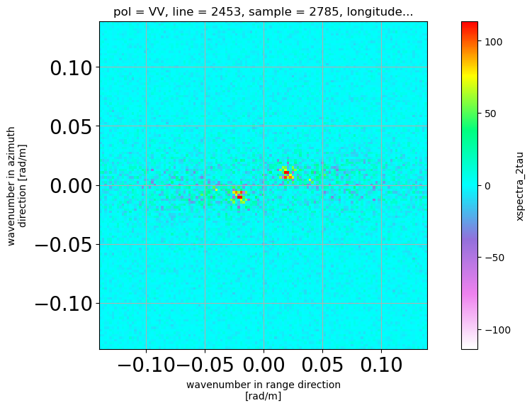
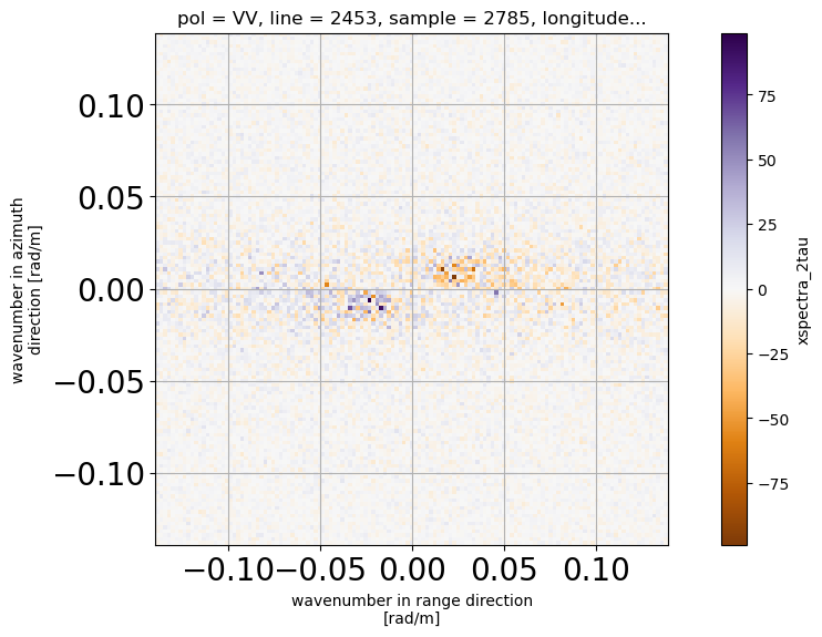
display difference with / without IR correction
[13]:
import numpy as np
from xsarslc.processing import xspectra
xs = xs0.swap_dims({'freq_line': 'k_az', 'freq_sample': 'k_rg'})
xs = xspectra.symmetrize_xspectrum(xs['xspectra_2tau'], dim_range='k_rg', dim_azimuth='k_az')

xs_ir = xs1.swap_dims({'freq_line': 'k_az', 'freq_sample': 'k_rg'})
xs_ir = xspectra.symmetrize_xspectrum(xs_ir['xspectra_2tau'], dim_range='k_rg', dim_azimuth='k_az')

############################################ real part ############################
coS=np.abs(xs.mean(dim='2tau').real) # co spectrum = real part of cross-spectrum
coS_reduced = coS.where(np.logical_and(np.abs(coS.k_rg)<=0.14, np.abs(coS.k_az)<=0.14), drop=True)

coS_IRcor=np.abs(xs_ir.mean(dim='2tau').real) # co spectrum = real part of cross-spectrum
coS_reduced_IRcor = coS_IRcor.where(np.logical_and(np.abs(coS_IRcor.k_rg)<=0.14, np.abs(coS_IRcor.k_az)<=0.14), drop=True)
from matplotlib import pyplot as plt
%matplotlib inline
from matplotlib import colors as mcolors
cmap = mcolors.LinearSegmentedColormap.from_list("", ["white","violet","mediumpurple","cyan","springgreen","yellow","red"])
PuOr = plt.get_cmap('PuOr')
plt.figure(figsize=(8,6))
plt.subplot(1,1,1)
#coS_reduced_av=coS_reduced.rolling(k_rg=3, center=True).mean().rolling(k_az=3, center=True).mean()
di = coS_reduced-coS_reduced_IRcor
print(di)
di.plot(cmap=cmap)

plt.grid()
plt.xticks(fontsize=20)
plt.yticks(fontsize=20)
plt.axis('scaled')


############################################ imag.part ############################
ims = xs.mean(dim='2tau').imag.squeeze()
xS_red = ims.where(np.logical_and(np.abs(ims.k_rg)<=0.14, np.abs(ims.k_az)<=0.14), drop=True)
ims_irCor = xs_ir.mean(dim='2tau').imag.squeeze()
xS_red_IRCor = ims_irCor.where(np.logical_and(np.abs(ims_irCor.k_rg)<=0.14, np.abs(ims_irCor.k_az)<=0.14), drop=True)
#xS_av=xS_red.rolling(k_rg=3, center=True).mean().rolling(k_az=3, center=True).mean()

plt.figure(figsize=(8,6))
plt.subplot(1,1,1)
(xS_red-xS_red_IRCor).plot(x='k_rg',cmap=PuOr)
plt.grid()
plt.xticks(fontsize=20)
plt.yticks(fontsize=20)
plt.axis('scaled')
<xarray.DataArray 'xspectra_2tau' (k_az: 133, k_rg: 133)>
array([[-3.30231023,  0.20230055,  3.24634354, ..., -0.28420991,
        -5.80216624, -0.82587412],
       [-1.03039672,  4.10552075,  0.85178918, ..., -1.66087963,
        -2.70627495,  3.32467915],
       [ 0.68772213,  0.37675369, -4.81396219, ..., -1.86558608,
         0.48049893, -1.52556207],
       ...,
       [-1.52556207,  0.48049893, -1.86558608, ..., -4.81396219,
         0.37675369,  0.68772213],
       [ 3.32467915, -2.70627495, -1.66087963, ...,  0.85178918,
         4.10552075, -1.03039672],
       [-0.82587412, -5.80216624, -0.28420991, ...,  3.24634354,
         0.20230055, -3.30231023]])
Coordinates:
  * k_az       (k_az) float64 -0.138 -0.1359 -0.1339 ... 0.1339 0.1359 0.138
  * k_rg       (k_rg) float64 -0.1382 -0.1361 -0.134 ... 0.134 0.1361 0.1382
    pol        <U2 'VV'
    line       int64 2453
    sample     int64 2785
    longitude  float64 130.9
    latitude   float64 -41.45
[13]:
(-0.13921871536677022,
 0.13921871536677022,
 -0.1390863226967172,
 0.1390863226967172)
[14]:
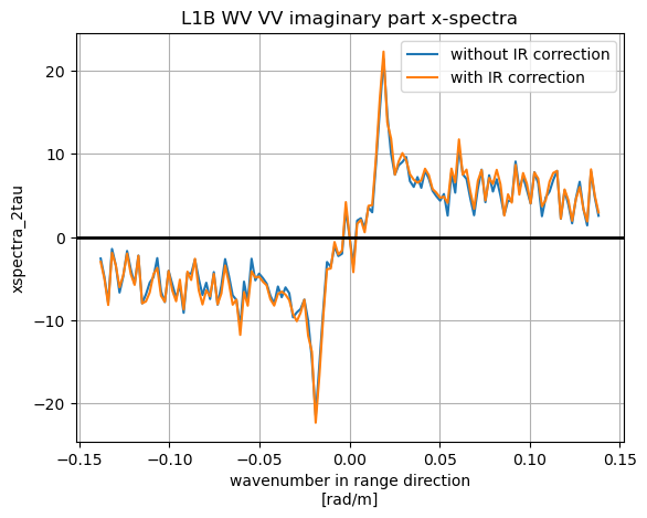
xS_red.mean(dim='k_az').plot(label='without IR correction')
xS_red_IRCor.mean(dim='k_az').plot(label='with IR correction')
plt.grid(True)
plt.legend()
plt.title('L1B WV VV imaginary part x-spectra')
plt.axhline(y=0,c='k',lw=2)
[14]:
<matplotlib.lines.Line2D at 0x7f57642aa8c0>